The hidden cost of running ClickHouse OSS at scale

ClickHouse OSS is remarkably easy to start. Put it on a large machine, point data at it, and it will take you surprisingly far.

The difficult part begins when one machine is no longer enough.

I have spent a lot of time operating self-managed ClickHouse clusters, and the costs that matter most rarely appear in the first infrastructure estimate. They emerge later: when a shard fills up, when another replica is needed, when replication falls behind, when Keeper becomes the coordination hot spot, or when a topology change turns into a migration project.

These are not bugs in ClickHouse. They are consequences of its shared-nothing architecture.

The shared-nothing bargain

#

In a typical self-managed ClickHouse cluster, each node owns local data and local compute. To store more data or use more CPU, you divide the dataset into shards. To survive failures or add read capacity, you create replicas of those shards.

The model is simple:

• Shards split the data.
• Replicas copy the data.
• Distributed tables route work across shards.
• ReplicatedMergeTree and ClickHouse Keeper coordinate replicas.

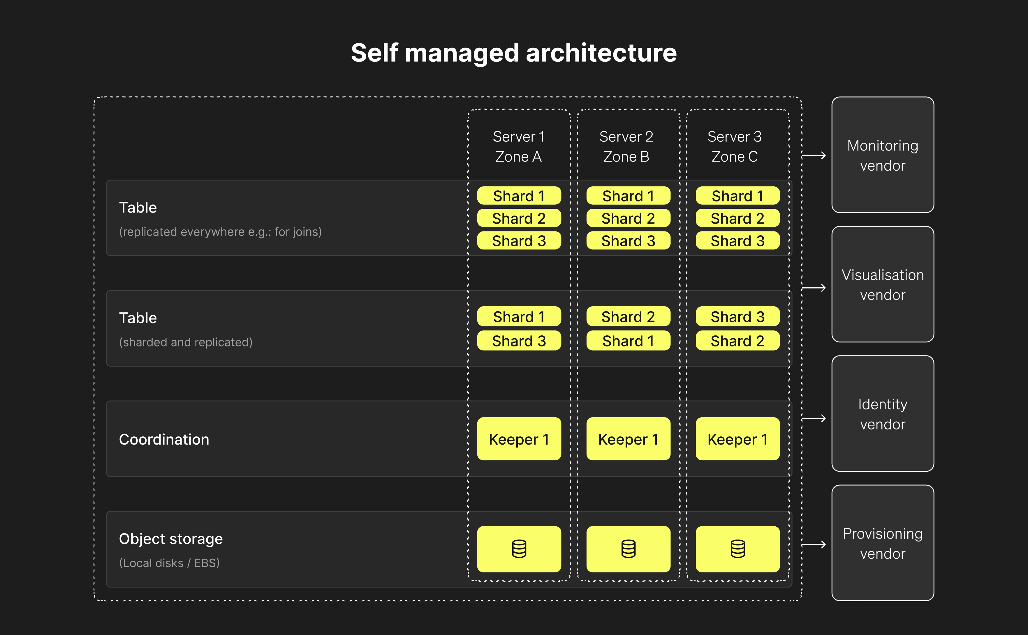
ClickHouse’s self-managed reference architecture. Source: ClickHouse Cloud architecture comparison.

This design performs well because computation happens close to local data. It also means that storage layout, compute capacity, and cluster topology are coupled. Adding a server is not the same as adding usable capacity.

That coupling is where the hidden cost starts.

Sharding makes scaling a data-placement problem

#

Suppose a cluster begins with one shard and two replicas. When the shard approaches its storage or compute limit, adding another shard does not automatically redistribute existing data.

There are two common reasons to add shards:

• Storage capacity: local disks are filling up, so the dataset has to be partitioned across more machines.
• Ingestion capacity: a single shard cannot parse, sort, compress, and merge incoming data fast enough, so writes have to be spread across more CPUs.

The second limit can arrive before the first. ClickHouse ingestion is often CPU-bound, especially with high row rates, expensive materialized views, complex codecs, or sustained background merges. Ingestion and queries then compete for the same CPU, memory bandwidth, and disk I/O. A node can have plenty of free storage while query latency deteriorates because writes and merges consume its compute budget.

Adding shards increases aggregate ingestion capacity by distributing that work. It also changes the data layout, however, so a compute bottleneck becomes a topology change rather than a simple CPU allocation. Adding replicas does not fully solve it either: replicas can increase read capacity, but each replica still performs replication work and background merges.

You now have to make several decisions:

• What is the new sharding key?
• Does historical data need to move?
• How will writes transition to the new topology?
• Can queries tolerate data living under two layouts during the migration?
• How do you validate that nothing was duplicated or missed?

Even when old data stays where it is and only new writes use the new shard, the cluster becomes less balanced over time. If data must be redistributed, scaling becomes an I/O-heavy migration with operational risk.

Query behavior changes too. A distributed query fans out to the relevant shards and waits for their results. One overloaded or unhealthy shard can determine tail latency for the entire query. The more shards a query touches, the more network calls and failure surfaces it acquires.

The hardware is only the visible cost. The hidden cost is designing, executing, observing, and sometimes rolling back the topology change.

Replicas multiply more than storage

#

Replicas are necessary for high availability and can increase read throughput, but a replica is not free compute attached to existing storage. It is another full copy of the shard.

Adding a replica means:

• Copying or fetching all of the shard’s data.
• Paying for another full set of disks.
• Running background merges on another server.
• Warming another local cache.
• Routing traffic so the extra read capacity is actually used.
• Monitoring replication queues and lag.
• Planning for the network and I/O load of recovery after a failure.

A cluster with two shards and two replicas already has four data-bearing nodes. Moving to four shards with two replicas doubles that footprint to eight. If storage and compute requirements grow at different rates, the topology cannot express that cleanly: scaling one often means paying for more of the other.

Replication also changes failure recovery. A replacement node may be easy to provision, but it is not useful until it has recovered enough data and cache state to serve the workload safely. At large data volumes, that recovery path deserves the same capacity planning as normal traffic.

It is worth being precise about the shape of this cost. shards × replicas is multiplicative, not mathematically exponential. If the replica count stays at two, doubling the shards doubles the data-node fleet:

What makes the bill feel worse than linear is the way capacity arrives in steps. A new shard normally brings its replicas, disks, cache, merge capacity, and failure-domain placement with it. The cluster is sized for the hottest shard and for failover, not for the average CPU graph. That leaves paid capacity idle between growth events.

The other dimension is read capacity. Replicas can serve independent queries when traffic is balanced across them, so a shard that is saturated by concurrent reads may need another replica even when it has enough storage and ingestion capacity. ClickHouse’s own concurrency sizing guidance makes an important distinction: replicas add read throughput, while parallel replicas allow a suitable single query to use multiple replicas. In the normal distributed path, simply adding a replica does not automatically make one query faster.

Technically, a team can add a third replica only to the hot shard. Operationally, that creates an asymmetric cluster: shards now have different read capacity, failure tolerance, cache state, and routing behavior. Many teams keep the topology uniform instead. Moving from two replicas to three then adds one complete copy of every shard:

That is the expensive step hidden behind “add read capacity.” A local problem on one shard can turn into M new servers because the production topology is kept symmetric. Each server needs the shard’s full data, performs replication and background merges, warms its own cache, and consumes recovery bandwidth. Going from two replicas to three is not a small adjustment; it increases the entire data-node fleet by 50%.

Keeper becomes part of the scaling boundary

#

ReplicatedMergeTree uses ClickHouse Keeper to coordinate replication metadata. Keeper does not store the table data itself, but it sits on the control path for replicated tables, parts, mutations, and other coordination work.

Once replication is introduced, the ClickHouse cluster is no longer the only system the team operates. Keeper needs its own odd-sized quorum, durable storage, backups, monitoring, upgrades, latency budgets, and failure procedures.

Adding replicas increases this burden as well as the data-node bill. Every new replica registers itself, maintains replication state and queues, watches metadata, reports part state, and participates in mutations and recovery. A change from 8×2 to 8×3 adds eight full ClickHouse servers, but those servers all attach to the same Keeper control plane.

The important limit is Keeper’s write path. Keeper uses Raft: clients can connect to different Keeper nodes, but writes are ordered through the current leader, appended to its log, and replicated to a quorum before they are committed. Followers improve availability; they do not create independent write leaders. Keeper write throughput is therefore bounded by the leader’s CPU and durable-log latency, plus the network and disk latency needed to reach a majority.

This makes coordination writes a finite cluster-wide budget. The ClickHouse replication documentation says that each inserted block creates approximately ten Keeper entries through several transactions. Small insert batches create more blocks, and therefore far more coordination work for the same number of rows. Frequent part creation, schema changes, mutations, replica churn, and recovery add traffic on top.

The rough shape is:

Keeper pressure =
  inserted blocks and part metadata
  + replicated tables × replicas
  + mutations and DDL
  + replica recovery and churn

Adding more Keeper quorum members does not scale that write path horizontally because there is still one leader. Scaling the ClickHouse data nodes does not remove the bottleneck either; it can send even more sessions, watches, and metadata operations toward the same leader.

ClickHouse supports auxiliary_zookeepers, which allows different tables to place their replication metadata in different Keeper or ZooKeeper clusters. This can partition the write load. It also changes one control plane into several:

• Another odd-sized Keeper quorum to provision and place across failure domains.
• Another set of disks, snapshots, alerts, certificates, and upgrade procedures.
• Configuration and credentials distributed to every ClickHouse node that uses it.
• A permanent table-to-Keeper mapping that operators must understand during incidents.
• More recovery and migration procedures to test.

That is a valid escape hatch for a very large deployment, but it is not free scale-out. Once Keeper has to be sharded by table, coordination capacity has become an architecture of its own, and the operational cost rises close to linearly with the number of Keeper clusters.

In practice, this creates another class of incidents to understand:

• Is replication slow because a replica is overloaded?
• Is the network dropping coordination requests?
• Is Keeper latency increasing?
• Are there too many parts or queued operations?
• Will restarting a node reduce pressure or trigger an expensive recovery?

Keeper is a solid coordination system. The hidden cost is that coordination itself becomes production infrastructure owned by your team.

The operational bill is larger than the server bill

#

The raw infrastructure comparison between ClickHouse OSS and ClickHouse Cloud is tempting: add up instances and disks, compare the number with the managed-service price, and declare self-hosting cheaper.

That comparison leaves out the work required to keep a shared-nothing cluster healthy:

• Capacity planning for each shard.
• Rebalancing and resharding.
• Replica placement across failure domains.
• Keeper operation and recovery.
• Backups and restore testing.
• Rolling upgrades across compatible versions.
• Configuration consistency across nodes.
• Monitoring merges, parts, queues, disks, and query fan-out.
• On-call time when any of these systems interact badly.

For a large, steady workload with an experienced platform team, self-managed ClickHouse can still be the right economic choice. But the honest cost is not just compute plus storage. It includes the engineering time and operational risk created by the topology.

What shared storage changes

#

ClickHouse Cloud uses SharedMergeTree: table data lives in shared object storage, while compute replicas process that data. The durable copy of the dataset is no longer tied to the lifecycle of an individual compute node. ClickHouse describes this as the progression from shared-nothing servers with local state to stateless compute over shared data.

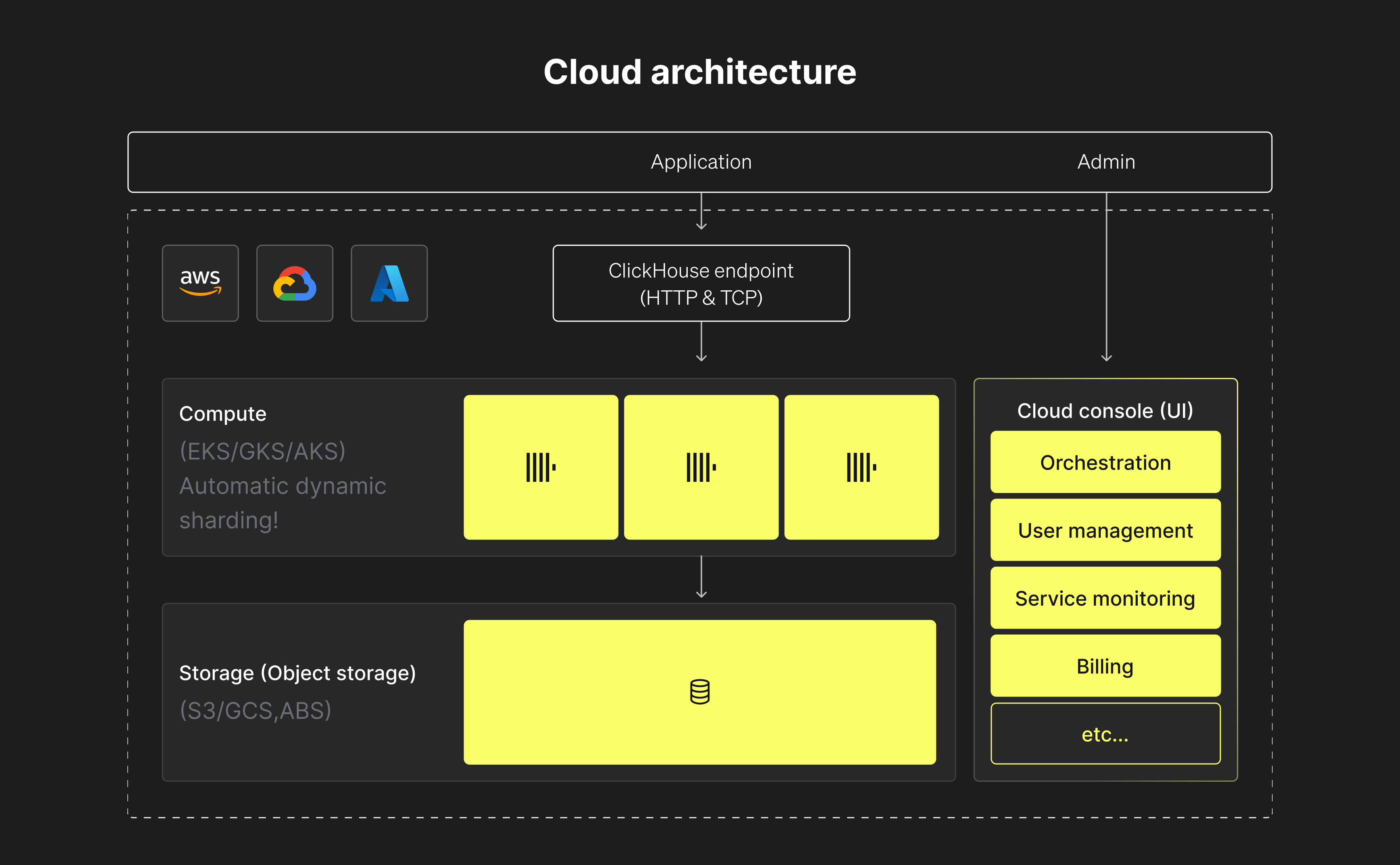
ClickHouse Cloud separates the compute fleet from shared object storage and adds a managed control plane. Source: ClickHouse Cloud architecture comparison.

That changes the scaling problem:

• Adding compute does not require creating another full durable copy of the data.
• Replacing a compute node does not require rebuilding the dataset from another replica.
• Storage and compute can grow more independently.
• Multiple compute services can use the same underlying data.
• Horizontal scaling does not require manually resharding the table first.

This does not make distributed systems disappear. New compute still needs CPU, memory, cache warm-up, and coordination. Object storage introduces its own latency and cost model. ClickHouse Cloud also charges a managed-service premium and gives the operator less control over versions, configuration, and infrastructure.

But it removes the coupling that matters for the cost model below: in shared-nothing OSS, storage, ingestion capacity, query capacity, and replication are expressed through the same fleet. In Cloud, they can be priced and scaled more independently.

A simple TCO estimate

#

Use one deliberately simple assumption: every compute node has 4 vCPU and 8 GB of memory. Baseline needs two compute nodes and retains 1 TB.

In this model, Cloud runs those two nodes over one shared copy of the data. The comparable production OSS topology uses two shards for the workload and two replicas for HA: four data nodes plus a separate three-node Keeper quorum.

The baseline monthly estimate is:

From 2 nodes to N

#

Let N be the number of Cloud compute nodes and D the retained logical data at that scale. There are two materially different OSS outcomes:

The good case is N×2. If queries prune cleanly and spread evenly across shards, every new shard adds ingestion, storage, and useful read capacity, while the replica count stays at two.

The bad case appears when queries are skewed, hot shards dominate, or query concurrency must scale independently of ingestion. Adding shards does not solve that problem, so replicas also grow. At R=N, an N-node Cloud service maps to N×N OSS data nodes, while S3 grows from one logical copy to N copies.

Keeper is not a fixed cost that disappears at large N. Its initial quorum cost is diluted for a while, but more shards, parts, replicas, and write activity increase coordination load. Keeper writes still pass through a leader; once that path is saturated, larger Keeper nodes or additional coordination domains add another step in both infrastructure and operational cost.

For example, if the workload and retained data double from the baseline, Cloud grows from 2 to 4 nodes and from 1 to 2 TB:

These are estimates, not quotes. They assume:

• A Cloud node at roughly $436/month, derived from the current AWS us-east-1 Scale price, plus shared storage at $25.30/TB-month.
• An OSS node at roughly $112/month for 4 vCPU and 8 GB, based on round EC2 On-Demand pricing.
• OSS data on S3 at roughly $23/TB-month. Each replica owns its own copy, so S3 data storage is approximately logical data × replica count; sharding partitions the logical dataset and does not multiply it again.
• Three Keeper nodes at $222/month for baseline, with twice the Keeper capacity budgeted for the larger replicated topology.
• One S3 backup copy of the logical dataset at $23/TB-month.
• Six OSS operational hours per month at $150/hour for the baseline.

Local cache disks, S3 request and transfer charges, and temporary or inactive parts are excluded. That makes the OSS estimate optimistic rather than punitive.

The real trade-off

#

The difference between ClickHouse OSS and ClickHouse Cloud is not simply free software versus a cloud bill.

It is a choice about where complexity lives.

With self-managed ClickHouse, the software is open and the infrastructure can be cheaper, but the user owns sharding, replication, coordination, recovery, and the people-hours behind them. With ClickHouse Cloud, more of that complexity is absorbed by the platform, and the premium appears directly on the invoice.

My practical rule is:

• Choose OSS when the workload is stable, the hardware will stay busy, and the team already has the operational capability.
• Choose Cloud when growth is uncertain, utilization is uneven, or avoiding topology and on-call work is more valuable than minimizing the raw infrastructure bill.

The decision should be revisited as the topology changes. A 1×2 cluster and an 8×2 cluster are not the same economic product, even if both are called “self-managed ClickHouse.”

After operating the OSS architecture, the question I keep coming back to is not whether shared storage is useful. It clearly is.

The more interesting question is whether we can get its decoupled scaling model without giving up the control and economics that make open-source ClickHouse attractive.

That is the architecture I want to explore next.